An overview of importance sampling techniques
- Numerical integration in 1D
- Multidimensional integrals & Monte Carlo
- Rejection sampling
- Stratified sampling
- Quasi Monte Carlo
- Importance sampling (IS)
- Multiple importance sampling (MIS)
- Weighted importance sampling (WIS - SNIS)
- Resampled importance sampling (RIS)
- Weighted reservoir sampling (WRS)
- Multiple weighted importance sampling (MWIS)
- To learn for the next time
1. Numerical integration in 1D 
Problem:
$I=\int_a^b f(x)\mathrm{d}x$
Solutions:
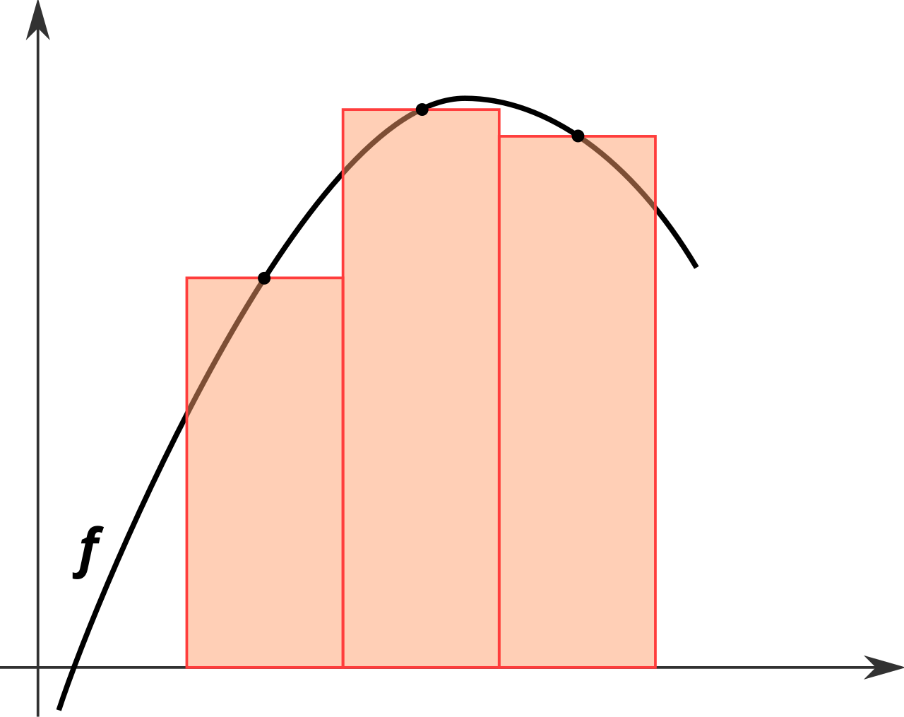
- Simple uniform quadratures: rectangles rule, trapezoidal rule, Simpson's rule = Piecewise polynomial interpolation
| Rectangle rule | Trapezoidal rule | Simpson's rule |
|---|---|---|
 |
 |
 |
(images from wikimedia)
- Superior orders uniform quadratures: Newton-Cotes, Romberg
- Weighted quadratures with non uniform subdivisions: Gaussian quadratures (Gauss - Legendre, ...)
- Other methods: for specific forms of integral (Laplace), adaptive methods, ...
Example 1.1: integrate the square function with the rectangle rule
$I=\int_0^2 x^2\mathrm{d}x$
Python function that performs the rectangle quadrature of $f$ on domain $[a,b]$ with $n$ subdivisions:
def rectangle_rule(f, a, b, n):
    size = (b - a) / n
    area_inf, area_sup = 0, 0
    for i in range (n):
        area_inf = area_inf + size * f(a + i * size)
        area_sup = area_sup + size * f(a + (i+1) * size)
    return area_inf, area_sup
2. Multidimensional integrals & Monte Carlo 
Problem:
- Multi dimensional integrals: surfaces/volumes integration, physics simulation, computer graphics simulation $\rightarrow$ rendering, games AI, ... and a lot more applications. $$ I = \int_{\Omega_0} \int_{\Omega_1} \dots \int_{\Omega_k} f(x_0, x_1, \dots, x_k) \prod_{i=0}^k \mathrm{d}x_i $$
- Can not be solved by quadratures efficiently (the number of samples grows exponentially
Solution:
- Monte carlo methods: approximate the integral by random sampling of the integration domain $$ I \approx \hat{I} = \frac{1}{n}\sum_{i=1}^n \frac{f(x_i)}{p(x_i)} $$
- $p(x)$ is the probability density function of the samples and has to be normalized $\int_\Omega p(x)dx = 1$
Downsides:
- Uniform sampling is (often) easy but MC estimators are noisy (variance) due to the random sampling process and require a large amount of samples to converge
- With pure random sampling the error vanishes in $O(\frac{1}{\sqrt n})$, hence it requires 4 times more samples to divide the error by 2
- Designing efficient and correct non uniform sampling is hard - (see. importance sampling section)
Your mission, should you choose to accept it: reduce the variance of the estimator at any cost
Example 2.1: integrate the square function with Monte Carlo
$I=\int_0^2 x^2\mathrm{d}x$
- Uniformly sample the domain $[0,2[$, with probability density $p(x)=\frac{1}{2}$

3. Rejection sampling 
Problem:
- When we do not know how to sample from distribution $g$
- But we know to sample from distribution $f$ such that $c \cdot f(x) > g(x)$
Solution:
- Sample larger than the target distribution domain
- And reject samples that are outside the region of interest
- Sampling routine:
- Sample $x$ from $f$
- Uniform sample $u$ in $U(0,1)$
- While $u > \frac{g(x)}{c \cdot f(x)}$ go to 1.
- Accept $x$ with probability density $g(x)$
(generic version replace $\frac{g(x)}{c \cdot f(x)}$ by $h(x)$ with values in $[0,1]$)
Pros: allow to sample arbitrary distributions from uniform samples
Cons: can be very inefficient if the proportion of rejection is greater than acceptance
Example 3.1: Estimate Pi with Monte Carlo and rejection sampling
- Sample $x$ uniformly in square((0,0), (2,2)), with pdf $p(x) = 1/4$
- $h(x) = 1$ if $x \in C$ else $h(x) = 0$ $\rightarrow$ binary acceptance
(modified animation from eduscol)
4. Stratified Sampling 
Problem:
- Classic uniform sampling suffers from void and cluster regions, how to get a better space coverage ?
Solution:
- Subdivide the domain and random sample in subregions
- Converges faster than uniform sampling
- Works in high dimensions since 2019 (cf. Orthogonal array sampling for Monte Carlo rendering)
Downside:
- Require covering the whole grid to get the correct estimation (the N-dimensionnal grid has a loooooot of cells)

Example 4.1: Estimate Pi with Monte Carlo, rejection sampling and stratified samples
(modified animation from eduscol)
5. Quasi Monte Carlo 
Problem:
- If noise comes from randomness, can we chose the random ? ... ... ... Yes !
Solution:
- Low discrepancy sequences
- Halton, Hammersley, Sobol, R2 / RN, Lattices
- Sequences are often designed to minimize the discrepancy (measure of space coverage)
- The error vanishes as fast as the discrepancy decreases
- e.g. Sobol error decrease with rate $O(1/n)$ $\rightarrow$ with 2 times more samples the error is divided by 2
- Optimized Pointsets
- Dart Throwing, BNOT, LDBN, SOT
- Pointsets are often designed to minimize the optimal tranport cost (but other measures exists)
- The error vanishes as fast as the optimal transport cost decreases
Comparison of LDS sequences (from Martin Roberts blog):
Comparison of pointsets (from utk and sot):
| Dart Throwing | BNOT | LDBN | SOT |
|---|---|---|---|
 |
 |
 |
 |
Downside:
- Don't mess up the points ... or they'll mess you
Example 5.1: Estimate Pi with Monte Carlo, rejection sampling and LDS samples
(modified animation from eduscol)
6. Importance sampling (IS) 
Problem:
- Uniform sampling puts samples everywhere even in unimportant areas
- What if the integrand is non zero over a small part of the domain ?
Solution:
- Put more samples in the important regions and correct the bias (correctly modify the probability density $p(x)$) = Non uniform distributions
- Dramatically reduces variance when it works (zero variance estimators exist)
- If the sample distribution is proportionnal to the integrand, $\frac{f(x)}{p(x)}=k$, then the MC estimator is a zero variance estimator = Perfect importance sampling: $$ \hat{I} = \frac{1}{n}\sum_{i=1}^n \frac{f(x)}{p(x)} = \frac{1}{n}\sum_{i=1}^n k = k \quad \text{and} \quad \mathbb{V}\left[\hat{I}\right]=0 $$
Downside:
- Can completely fail ...

- How to chose or design a (biased) perfect non uniform distribution is hard, several methods exists such as:
- the inverse CDF method (analytic or numeric, e.g. triangle cut method),
- warping by a transformation (analytic or numeric),
- rejection sampling,
- generic model + learning,
- others I do not know yet ...
- e.g. the first example integrand $f(x)=x^2$ is hard to importance sample analytically (but rejection or numerical methods are available)
Example 6.1: integration of a Gaussian, uniform VS importance sampling

7. Multiple importance sampling (MIS) 
Problem:
- Several importance sampling strategies available $p_1, p_2, \dots, p_k$
- How to combine the associated estimators $\hat{I}_1,\hat{I}_2, \dots, \hat{I}_k$ ?
- Average is not better than individual estimators (per estimator weight)
- Use a weighted mixture of sampling strategies instead (per sample weight) $\rightarrow$ MIS
Solution:
- Multi Sample Model distribute a fixed number of samples $n_i$ per strategy and weight contributions: $$ \hat{I}_{\text{ms-mis}}=\sum_{i=1}^{k} \hat{I}_i = \sum_{i=1}^{k} \frac{1}{n_i}\sum_{j=1}^{n_i} \color{red}{w_i(x_{ij})}\frac{f(x_{ij})}{p_i(x_{ij})} $$
- One Sample Model distribute one sample from strategy selected with fixed probability $c_i$ and weight contributions: $$ \hat{I}_{\text{os-mis}}=\frac{1}{N}\sum_{j=1}^{N} \color{red}{w_i(x_{ij})}\frac{f(x_{ij})}{c_i p_i(x_{ij})} $$
Condition on weighting functions: $\sum_i w_i(x) = 1$, in practice balance heuristic weights are a provably good solution: $$ w_i(x) = \frac{c_i p_i(x)}{\sum_{j=1}^{k} c_j p_j(x)} $$ Downside:
The strategy of highest density is preponderant
- What if the distribution is a bad importance sampler regarding the integrand ?
- Still dominant weights on unimportant parts of the domain $\rightarrow$ more variance
- Several references propose improvements over Veach MIS: Variance aware MIS, Optimal MIS,...
Example 7.1: integration 1D
- Complex multi term integrand: $f(x) = \frac{\exp{\frac{-x^2}{50}} \cdot \left|x\right| \cdot \left(\cos{x}+1\right)}{5}$
- Sampling with two gaussians under peaks and uniform sampling as a defensive strategy
- Equal sample count per strategy

Example 7.2: Direct illumination sampling with Veach MIS
| BSDF sampling | Light sampling | MIS |
|---|---|---|
 |
 |
 |
(images from Yining Karl Li blog)
8. Weighted importance sampling (WIS - SNIS) 
Problem:
- What if we know how to sample from distribution $q$ but want to evaluate the estimator w.r.t $p$ ? (target density $\neq$ source density)
Solution:
“If we really accepted the idea that a sample from one distribution is a sample from any distribution (if appropriately weighted) then we should not be surprised at the next two results stated below.” - Trotter and Tukey - Conditional Monte Carlo For Normal Samples - 1954
Estimate both the integral and the bias correction term at once, and use a ratio of integrals: $$ I = \int_\Omega f(x)\mathrm{d}\mu(x) = \mathbb{E}\left[\frac{f(x)}{p(x)}\right] = \mathbb{E}\left[\frac{f(x)}{q(x)}\frac{q(x)}{p(x)}\right] \qquad \approx \qquad \frac{\mathbb{E}\left[\frac{f(x)}{q(x)}\right]}{\mathbb{E}\left[\frac{p(x)}{q(x)}\right]} = \frac{\mathbb{E}\left[w(x)\frac{f(x)}{p(x)}\right]}{\mathbb{E}\left[w(x)\right]} \quad \text{with} \quad w(x)=\frac{p(x)}{q(x)} $$
The associated self normalizing Monte Carlo estimator (ratio estimator) can be estimated using a weighted mean: $$ \tilde{I} = \frac{ \frac{1}{n} \sum_{i=1}^n w(x_i)\frac{f(x_i)}{p(x_i)} }{ \frac{1}{n} \sum_{i=1}^n w(x_i)} = \frac{ \sum_{i=1}^n w(x_i)\frac{f(x_i)}{p(x_i)} }{ \sum_{i=1}^n w(x_i)} $$
The closer $p$ is to the perfect importance distritbution w.r.t the integrand, the better will be the estimator (can reach 0 variance if $f(x)=kp(x)$)
Downside:
- Biased but consistent, the bias can be perceived at low sample count, but tends towards 0 as number of samples increase
Example 8.1: integration with WIS

9. Resampled importance sampling (RIS) 
Problem:
- Can we get rid of the bias in WIS ? ... ... ... yes, via discrete random resampling !
Solution:
- Importance Resampling for Global Illumination , Talbot et al., 2005
- Generate a set of $M$ samples from $q$ and select one sample with discrete resampling
- Sampling routine:
- Generate $M$ candidates samples from $q$
- Eval for each candidate $x_i$ the resampling weight $w(x_i)=\frac{p(x_i)}{q(x_i)}$
- Build the discrete CDF of the sample weights (covered in Ray Tracing Gems - Chapter 16.3.4)
- Random sample the discrete CDF to get a single sample approximately distributed from $p$: $$ \begin{split} p_{\text{RIS}}(x_i) &= \frac{q(x_i)w(x_i)}{\frac{1}{M}\sum_{j=1}^M w(x_j)} \qquad \text{with} \qquad \quad w(x)=\frac{p(x)}{q(x)} \\ &=\frac{p(x_i)}{\underbrace{\frac{1}{M}\sum_{j=1}^M w(x_j)}_{\text{bias correction term}}} \end{split} $$
- The number of candidates $M$ interpolates from distribution source $q$ ($M=1$) to target distribution $p$ ($M=\infty$)
- The resampling weight in the pdf is a bias correction term, hence we use the classic unbiased Monte Carlo estimator: $$ \hat{I} = \frac{1}{n}\sum_{i=1}^n \frac{f(x_i)}{p_{\text{RIS}}(x_i)} $$
Downside:
- Impractical if $q$ is complex/costly to sample, generating $M$ candidates is be a waste of computational time
Example 9.1: 1D RIS approximated density comparison

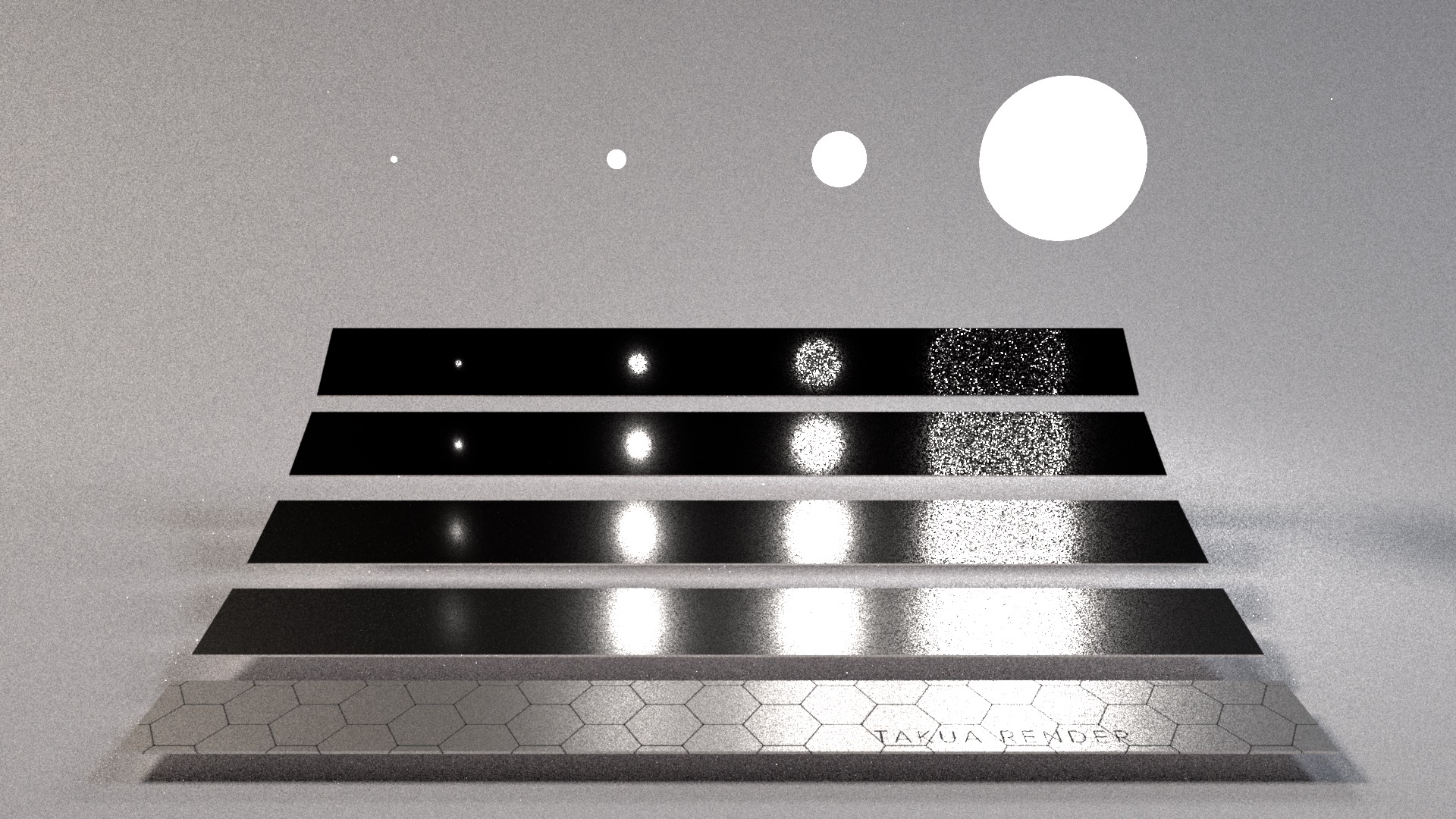
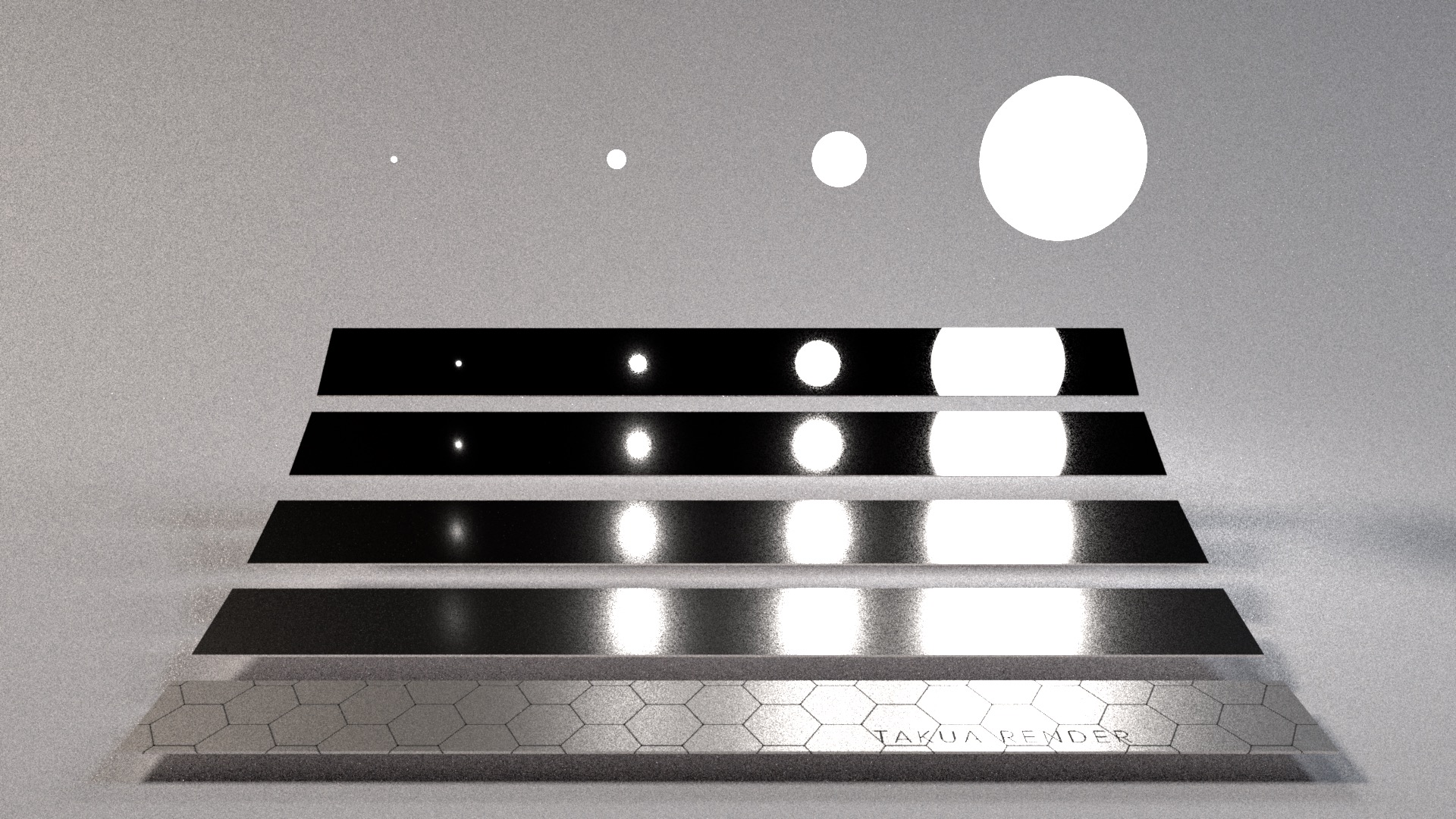
Example 9.2: direct illumination sampling with RIS
| Scene (left half RIS, right half IS) | Light sources area RIS - 8 candidates | Light sources area IS |
|---|---|---|
 |
 |
 |
10. Weighted reservoir sampling (WRS) 
Problem:
- Can we resample from a stream of samples without
- building the discrete CDF
- storing all samples
- knowing the number of samples to be drawn ?
- Again ... yes !
Solution:
- Spatiotemporal reservoir resampling for real-time ray tracingwith dynamic direct lighting , Bitterli et al., 2020
- Use a reservoir $R(x, w, s)$
- Reservoir resampling routine for each sample:
- Sample $x_i$ from $q$
- Eval the resampling weight $w(x_i)=\frac{p(x_i)}{q(x_i)}$
- Update the sum of weights in the reservoir with the new sample weight $s=s+w(x_i)$
- Try to replace the sample currently in the reservoir by the new sample with probability $c_i=\frac{w(x_i)}{s}$
- If the sample is accepted, the stored sample and weight in the reservoir are modified accordingly: $x=x_i \quad w=w(x_i)$
- WRS = RIS without storing all candidates, inversing the cdf, knowing the number of candidates (does not appear in the pdf anymore)
- WRS is covered in Ray Tracing Gems II - Chapter 22)
Downside:
- Impractical if $q$ is complex/costly to sample, generating $M$ candidates is be a waste of computational time
Example 10.1: Reconstructed density with WRS (similar to RIS)
The figure below shows several kernel density reconstruction over 10000 RIS samples.
The initial samples are distributed from the uniform distribution (orange), and resampled using different number of candidates $M$ to approximate a target gaussian density (blue).
Increasing the number of candidates leads to a better approximation of the target density, at the expense of sampling more candidates.

Example 10.2: Direct illumination sampling in real time ray tracing application (combine RIS and WRS)
- Multiple strategies RIS combined with reservoir sampling (see next section) has been recently explored for direct illumination sampling in real time ray tracing applications - cf. Spatiotemporal reservoir resampling for real-time ray tracingwith dynamic direct lighting

(from ReSTIR project page)
11. Multiple weighted importance sampling (MWIS) 
Problem:
- WIS + multiple strategies $q_1, \dots, q_k$ = MWIS ?
Solution:
- Volumetric Multi-View Rendering, Fraboni et al., 2021
- Combine WIS and MIS in a single self normalizing ratio estimator (ratio of sum of integrals comparable to the MIS formulation as a sum of integrals):
- The combined weighting function is defined as: $$ w_{i,\text{mwis}}(x)=w_{i,\text{mis}}(x) \cdot w_{i,\text{wis}}(x) $$
- Which is a valid weighting heuristic within the MWIS framework thanks to the self-normalization of the estimator ($\sum_{j=1}^k w_{j,\text{mwis}}(x) \neq 1$)
- The associated Monte Carlo estimator using reduces to a weighted mean of samples:
- Combine any number of strategies to reconstruct any distribution; Wouhou as generic as can be !
- Application in path reusing algorithms
Downside:
- Same as WIS, biased but consistent estimator
Example 11.1: multi-view rendering with the MWIS estimator
- Sequence of N frames, reuse path sampled from other cameras to reduce the variance of the whole sequence
- Instead of rendering frames separately, we render the whole sequence at once
- The process of reusing a path is unknown a priori $\rightarrow$ use of MWIS to reduce the variance of reusing path that can not contribute
- Can work with animated scenes: reuse path at fixed time, overlap shutter windows of cameras $\rightarrow$ variance reduction in motion blur
TODO: add images and examples 1D - 2D
12. To learn for the next time 
- Markov Chain Monte Carlo; it is easier without pdfs ¯\_(ツ)_/¯
- idea: start from a random sample, try some random mutations on the sample, accept the mutation with probability $\alpha=\frac{f(x_{i+1})}{f(x_i)}$, after a lot of mutations the target distribution is reproduced
- Metropolis, Primary Sample Space Metropolis, Reversible Jump Metropolis, Monte Carlo Langevin (Metropolis + Gradient), Hamiltonian Monte Carlo (Metropolis + Moments),...
- Adaptive importance sampling; learn the pdf
- idea: start from proposal pdfs $q_i$ and iteratively refine them during the integration to match a target distribution $p$ (multi stage methods)
- Cross Entropy
- Population Monte Carlo
- Piecewise AIS: Vegas, ...
- Control Variates; learn (a part) of the estimator
- idea: use an unbiased estimation of $I$ to reduce the error of the estimator
- often multi stage to estimate the parameters that allow the error reduction
- Antithetic variates
- idea: take antithetics samples ($u'=1-u$) to reduce the variance of the estimator
- Still, there is room for improving and finding new applications using self normalized ratio estimators (WIS, MWIS, others), which have been shunned in offline rendering applications:
“Why did offline-rendering people publish several papers on control variates and (to our knowledge) never published a ratio estimator, which is simpler and better?” - Eric Heitz - Combining analytic direct illumination and stochastic shadows - 2018
Compile Jupyter to HTML:
jupyter nbconvert presentation.ipynb --no-input --to html --template full --no-prompt